• Introduction
• TD(0)
  • Example: Random walk
    • Code
    • Results
• SARSA: On policy TD Control
  • Example: Windy grid world
    • Code
    • Results
• Q-learning: Off-policy TD Control
  • Example: Cliff walking (Q-learning version)
    • Code
    • Results
  • Example: Cliff walking (SARSA version)
    • Code
    • Results
• References

Introduction

Temporal-difference (TD) learning is a combination of Monte Carlo ideas and dynamic programming (DP) ideas. Like Monte Carlo methods, TD learns from experience without needing the model of the environment’s dynamics. Like DP methods, TD learn estimates from other estimates (bootstrapping) without waiting for final outcome.

TD(0)

\(\begin{aligned} &V(S)\leftarrow V(S)+\alpha(R+\gamma V(S')-V(S))\\ &where \ S:State, V(S): value\ of\ state, R: observed\ reward\ for\ taking\ action,\\ &S':next\ state, \alpha: step\ size\ parameter ,\gamma: discount\ rate\\ \end{aligned}\)

To gain an intuition about the above equation, consider the following.

If V(S') $\uparrow$, increase value of current state V(S)

i.e. if the value of the next state S’ is better than the current state, increase the value of current state as this path leads to a next state of a higher value.

If R $\uparrow$, increase value of current state V(S)

i.e. if current breadcrumb path leads to higher reward, increase value of current state V(S) as it leads to a higher reward path.

Example: Random walk

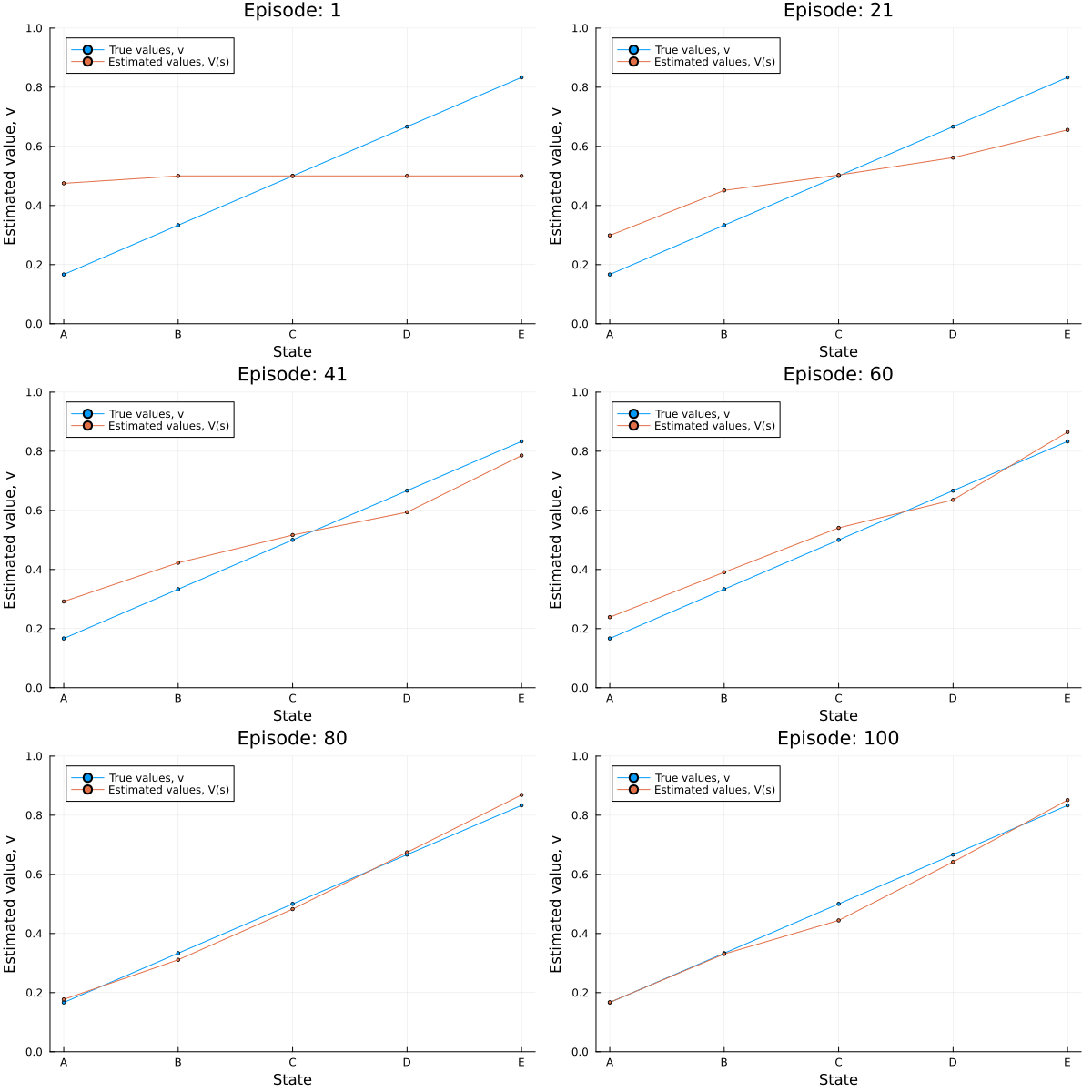
All episodes start in the center state, C, and proceed either left or right by one state on each step, with 0.5 probability. The episode terminates when either T1 or T2 is reached. A reward of +1 occurs when T2 is reached, all other rewards are 0.

Code

# TD(0) algorithm
# Random walk
# T1 <- A <-> B <-> C <-> D <-> E -> T2
using Plots
using Random
rng = Xoshiro(99)

function td0_random_walk(alpha = 0.05, viz = false)
    # Policy: random next state. 
    # true state values
    v = [1/6, 2/6, 3/6, 4/6, 5/6]
    err = []
    V_array = []

    # Init step
    # Reward
    R = Dict("T1" => 0, "A" => 0, "B" => 0, "C" => 0, "D" => 0, "E" => 0, "T2" => 1); 
    # Estimated value function
    V = Dict("A" => 0.5, "B" => 0.5, "C" => 0.5, "D" => 0.5, "E" => 0.5, "T1" => 0, "T2" => 0)  
    
    gamma = 1

    # Build graph
    Grp = Dict("A" => ["T1","B"], "B" => ["A","C"], "C" => ["B","D"], "D" => ["C","E"], "E" => ["D","T2"])

    for episode = 1:100 
        # init state 
        S = "C"
        while S != "T1" && S != "T2"
            # print(S,"->")
            # action: take probability of next step
            Snext = rand(rng, Grp[S])
            # check reward of next state
            reward = R[Snext]
            # update: V
            V[S] = V[S] + alpha*(reward + gamma * V[Snext] - V[S])
            # update: S to next state 
            S = Snext
        end

        push!(err, RMSE([V["A"], V["B"], V["C"], V["D"], V["E"]], v))

        # saves animation plot points
        if viz == true
            push!(V_array, [V["A"], V["B"], V["C"], V["D"], V["E"]])
        end

    end

    if viz == true
        # animation plot
        anim = @animate for i ∈ 1:length(V_array)
            plot(["A", "B", "C", "D", "E"], [v V_array[i]], 
            marker = 2, label = ["True values, v" "Estimated values, V(s)"], 
            xlabel="State", ylabel="Estimated value, v", ylims = (0,1),
            title = "Episode: $i")
        end
        gif(anim, "td0_random_walk.gif")
    end

    return err
end

# Root mean square error
function RMSE(estimate, truth)
    s = 0
    for i = 1:length(truth)
        s += (truth[i] - estimate[i])^2
    end
    return sqrt(1/length(truth)*s)
end

Results

# Generates gif animation
td0_random_walk(0.05, true);

err0 = td0_random_walk(0.05);
err1 = td0_random_walk(0.1);
err2 = td0_random_walk(0.15);

plot([err0 err1 err2], title = "RMS error vs episodes", label=["\\alpha=0.05" "\\alpha=0.1" "\\alpha=0.15"], xlabel = "Episodes", ylabel = "RMS error")

SARSA: On policy TD Control

SARSA learns the action-value function rather than the state-value function. This ‘on-policy’ learns $q_\pi(s,a)$ for a given policy $\pi$ for all states $s$ and action $a$.

SARSA algorithm

$$\begin{aligned} &Initialize\ Q(s,a),\forall\ s \in \mathbb S,\ a \in \mathbb A(s)\ arbitrarily,\ Q(terminal,.)=0\\ &For\ each\ episode\\ &\qquad Initialize\ S\\ &\qquad Choose\ A\ from\ S\ with\ policy\ \pi\ (e.g. \epsilon-greedy)\\ &\qquad For\ each\ step\ in\ episode\\ &\qquad \qquad Take\ Action\ A,\ Observe\ Reward\ R,\ next\ state\ S'\\ &\qquad \qquad Choose\ Action\ A'\ from\ next\ state\ S'\ with\ \pi\\ &\qquad \qquad Q(S,A) \leftarrow Q(S,A)+\alpha[R+\gamma Q(S',A')-Q(S,A)]\\ &\qquad \qquad S \leftarrow S', A \leftarrow A'\\ &\qquad until\ terminal\ S \end{aligned}$$

Example: Windy grid world

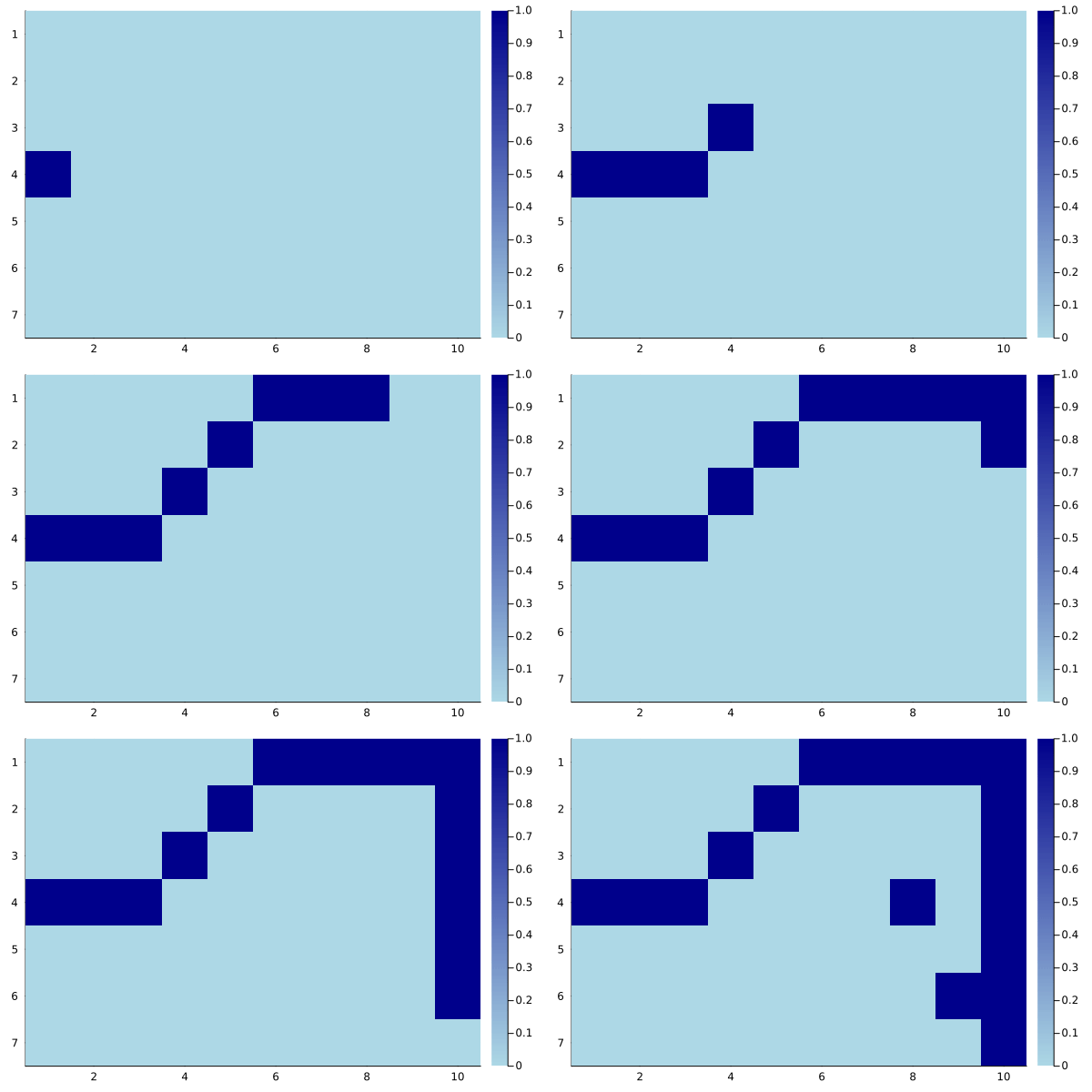
In windy grid world, we have a start position S and goal position G. There is a crosswind upward through the middle of the grid. The actions are the standard four moves: up, down, left, right but in the middle region the resultant next states are shifted upward by a “wind,” the strength denoted by the numbers at the bottom of the grid. Assume that moves at the edges of the grid world are not valid states.

Code

using Random, Distributions, Plots
Random.seed!(123)

alpha = 0.5
gamma = 1
max_row = 7   # max grid rows
max_col = 10  # max grid columns
start = (4,1) # start position
goal = (4,8)  # goal position
# set all positions to -1 reward except goal 
reward = -1 * ones(max_row, max_col)  
reward[goal...] = 0 # set goal reward to 0

# action A: up, down ,left, right
# policy π: epsilon - greedy
# upward wind - north bias vector [0 0 0 1 1 1 2 2 1 0] 
wind = [0 0 0 1 1 1 2 2 1 0]

# build valid state actions
sa = Dict()
for r = 1:max_row
    for c = 1:max_col
        valid_actions = []
        # left 
        if 1 <= c-1
            push!(valid_actions, (r,c-1))
        end
        # right 
        if c+1 <= max_col
            push!(valid_actions, (r,c+1))
        end
        # up
        if 1 <= r-1 
            push!(valid_actions, (r-1,c))
        end
        # down
        if r+1 <= max_row 
            push!(valid_actions, (r+1,c))
        end
        sa[(r,c)] = valid_actions

    end
end

# Initialise Q(s,a) = 0 for all s, a
Q = Dict()
for k = keys(sa)
    for v = 1:length(sa[k])
        Q[(k,sa[k][v])] = 0.0
    end
end

# epsilon greedy function
function epsilon_greedy(state, state_action, Q, epsilon)
    greedy_action = nothing
    greedy_action_value = 0.0

    # With probability epsilon pick a random action, with probability 1-epsilon take greedy action
    d = Bernoulli(epsilon)
    sample = rand(d, 1)

    if sample == Bool[1] 
        # Random action
        greedy_action = rand(state_action[state])

    else
        # Greedy action by picking action with maximum Q values
        for action in state_action[state]
            if greedy_action == nothing
                greedy_action = action
                greedy_action_value = Q[state, action] 
            else
                if Q[state, action] > greedy_action_value
                    greedy_action = action
                    greedy_action_value = Q[state, action]
                end 
            end
        end
    end

    return greedy_action
end

step_data = []
step_data2 = []
steps2 = 0

for episode = 1:200
    # Initialise state s, reward
    s = start
    r = 0
    steps = 0
    # Choose action for state with policy π
    a = epsilon_greedy(s, sa, Q, 0.1)

    while true
        # take action a, observe reward r, next state s'
        s_next = (max(1, a[1] - wind[a[2]]), a[2] )   # max op covers hitting north wall case, wind bias added
        r = reward[s...]

        # choose a' from s' with policy π
        a_next = epsilon_greedy(s_next, sa, Q, 0.1)
        
        # update Q
        Q[s,a] = Q[s,a] + alpha * (r + gamma * (Q[s_next,a_next] - Q[s,a]) )

        # update action and state
        s = s_next
        a = a_next

        steps += 1
        steps2 += 1
        if s == goal
            #println(steps)
            push!(step_data, steps)
            push!(step_data2, steps2)
            #println(Q)
            break
        end
        #print(s,"->")
    end
end

Results

println("Min steps found: ", minimum(step_data))
display(plot(step_data, xlabel = "Episode", ylabel = "No. of steps"))
display(plot(step_data2, xlabel = "Episode", ylabel = "Cumulative Time steps"))

Output:

Min steps found: 17

travelled_path = [start]

# Initialise state s, reward
s = start
steps = 0
# Choose action for state with policy π
a = epsilon_greedy(s, sa, Q, 0)  # set epsilon to 0 (greedy action)!!

while true
    # take action a, observe reward r, next state s'
    s_next = (max(1, a[1] - wind[a[2]]), a[2] )   # max op covers hitting north wall case, wind bias added

    # choose a' from s' with policy π
    a_next = epsilon_greedy(s_next, sa, Q, 0)   # set epsilon to 0 (greedy action)!!

    # update action and state
    s = s_next
    a = a_next

    push!(travelled_path, s) 
    steps += 1
    if s == goal
        println(steps)
        break
    end
    
end

gridplot_anim = zeros(max_row, max_col) 
windy_anim = @animate for path in travelled_path
    gridplot_anim[path...] = 1
    (heatmap(gridplot_anim, yflip=true, color=:blues))
end
gif(windy_anim, "windy_gridworld.gif", fps = 5) 

Q-learning: Off-policy TD Control

In Q-learning, the learned action-value function, Q, directly approximates $q_∗$ the optimal action-value function, independent of the policy being followed. The policy still has an effect in determining which state-action pairs are visited and updated. As long as all pairs are updated, convergence is achieved.

Q-learning algorithm

$$\begin{aligned} &Initialize\ Q(s,a),\forall\ s \in \mathbb S,\ a \in \mathbb A(s)\ arbitrarily,\ Q(terminal,.)=0\\ &For\ each\ episode\\ &\qquad Initialize\ S\\ &\qquad For\ each\ step\ in\ episode\\ &\qquad \qquad Choose\ A\ from\ S\ with\ policy\ \pi\ (e.g. \epsilon-greedy)\\ &\qquad \qquad Take\ Action\ A,\ Observe\ Reward\ R,\ next\ state\ S'\\ &\qquad \qquad Q(S,A) \leftarrow Q(S,A)+\alpha[R+\gamma max_a Q(S',a)-Q(S,A)]\\ &\qquad \qquad S \leftarrow S'\\ &\qquad until\ terminal\ S \end{aligned}$$

In the algorithm, we are $\boldsymbol{NOT}$ updating action A. Unlike SARSA, the action (e.g. action with max Q) is not followed in the next step - e.g. we are still running $\epsilon$-greedy for the next action. i.e. It does not account for action selection.

Example: Cliff walking (Q-learning version)

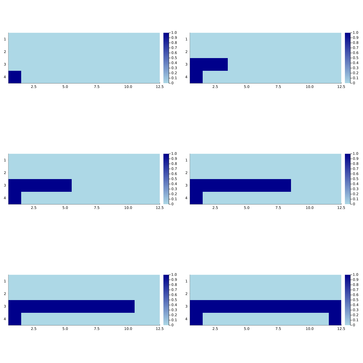
Again denote start point S and goal G. Movements are up, down, left, right. Rewards are 0 for the goal, -100 for the cliff areas and -1 elsewhere. Any travesal through the cliff areas sends the agent back to the start point S.

Code

using Random, Distributions, Plots
Random.seed!(123)

alpha = 0.5
gamma = 1
max_row = 4   # max grid rows
max_col = 12  # max grid columns
start = (4,1) # start position
goal = (4,12)  # goal position
# set all positions to -1 reward except goal 
reward = -1 * ones(max_row, max_col)  
reward[goal...] = 0 # set goal reward to 0
reward[4,2:11] .= -100 # set cliff reward to -100

# Q-learning for cliff walking
# action A: up, down, left, right
# policy π: epsilon - greedy

# build valid state actions
function build_state_action(max_row, max_col)
    sa = Dict()
    for r = 1:max_row
        for c = 1:max_col
            valid_actions = []
            # left 
            if 1 <= c-1
                push!(valid_actions, (r,c-1))
            end
            # right 
            if c+1 <= max_col
                push!(valid_actions, (r,c+1))
            end
            # up
            if 1 <= r-1 
                push!(valid_actions, (r-1,c))
            end
            # down
            if r+1 <= max_row 
                push!(valid_actions, (r+1,c))
            end
            sa[(r,c)] = valid_actions

        end
    end

    # cliff case 
    for i = 2:max_col-1
        sa[(4,i)] = Any[(4,1)]
    end
    return sa
end

sa = build_state_action(max_row, max_col)

# Initialise Q(s,a) = 0 for all s, a
Q = Dict()
for k = keys(sa)
    for v = 1:length(sa[k])
        Q[(k,sa[k][v])] = 0.0
    end
end

# epsilon greedy function
function epsilon_greedy(state, state_action, Q, epsilon)
    greedy_action = nothing
    greedy_action_value = 0.0

    # With probability epsilon pick a random action, with probability 1-epsilon take greedy action
    d = Bernoulli(epsilon)
    sample = rand(d, 1)

    if sample == Bool[1] 
        # Random action
        greedy_action = rand(state_action[state])

    else
        # Greedy action by picking action with maximum Q values
        for action in state_action[state]
            if greedy_action == nothing
                greedy_action = action
                greedy_action_value = Q[state, action] 
            else
                if Q[state, action] > greedy_action_value
                    greedy_action = action
                    greedy_action_value = Q[state, action]
                end 
            end
        end
    end

    return greedy_action
end

step_data = []
av_reward = []


for episode = 1:100
    # Initialise state s, reward
    s = start
    r = 0
    steps = 0
    reward_counter = 0
    while true
        # Choose action for state with policy π
        a = epsilon_greedy(s, sa, Q, 0.1)
        # take action a, observe reward r, next state s'
        s_next = a
        r = reward[s...]

        # choose a' from s' which returns max Q value 
        a_next = epsilon_greedy(s_next, sa, Q, 0)   # epsilon = 0 is greedy action by taking action with max Q
        
        # update Q
        Q[s,a] = Q[s,a] + alpha * (r + gamma * (Q[s_next,a_next] - Q[s,a]) )

        # update state. No update to action!
        s = s_next

        steps += 1
        reward_counter += r
        if s == goal
            #println(steps)
            push!(step_data, steps)
            push!(av_reward, reward_counter)
            #println(Q)
            break
        end
        #print(s,"->")
    end
end

Results

max_reward = maximum(av_reward)
println("Min steps found: ", minimum(step_data))
display(plot(step_data, xlabel = "Episode", ylabel = "No. of steps"))
display(plot(av_reward, xlabel = "Episode", ylabel = "Reward", label = "\$max\\: reward=$max_reward\$"))

Output:

Min steps found: 13

travelled_path = [start]

# Initialise state s, reward
s = start
steps = 0

while true
    # Choose action for state with policy π
    a = epsilon_greedy(s, sa, Q, 0)  # set epsilon to 0 (greedy action)!!
    # take action a, observe reward r, next state s'
    s_next = a

    # choose a' from s' which returns max Q value 
    a_next = epsilon_greedy(s_next, sa, Q, 0)   # set epsilon to 0 (greedy action)!!

    # update action and state
    s = s_next

    push!(travelled_path, s) 
    steps += 1
    if s == goal
        println(steps)
        break
    end
    
end

gridplot_anim = zeros(max_row, max_col) 
cliff_qlearning_anim = @animate for path in travelled_path
    gridplot_anim[path...] = 1
    (heatmap(gridplot_anim, yflip=true, color=:blues, aspect_ratio=:equal, ylimits=(0.5,4.5)))
end
gif(cliff_qlearning_anim, "cliff_q_learning.gif", fps = 5) 

We see that Q-learning learns to travel along the cliff (‘risky area’) to get to goal.

Example: Cliff walking (SARSA version)

Code

# Sarsa version of cliff walking

sa = build_state_action(max_row, max_col)

# Initialise Q(s,a) = 0 for all s, a
Q = Dict()
for k = keys(sa)
    for v = 1:length(sa[k])
        Q[(k,sa[k][v])] = 0.0
    end
end

step_data = []
av_reward = []

for episode = 1:100
    # Initialise state s, reward
    s = start
    r = 0
    steps = 0
    reward_counter = 0
    # Choose action for state with policy π
    a = epsilon_greedy(s, sa, Q, 0.1)
    while true
        # take action a, observe reward r, next state s'
        s_next = a
        r = reward[s...]

        # choose a' from s' with policy π
        a_next = epsilon_greedy(s_next, sa, Q, 0.1)
        
        # update Q
        Q[s,a] = Q[s,a] + alpha * (r + gamma * (Q[s_next,a_next] - Q[s,a]) )

        # update action and state
        s = s_next
        a = a_next

        steps += 1
        reward_counter += r
        if s == goal
            #println(steps)
            push!(step_data, steps)
            push!(av_reward, reward_counter)
            #println(Q)
            break
        end
        #print(s,"->")
    end
end

Results

max_reward = maximum(av_reward)
println("Min steps found: ", minimum(step_data))
display(plot(step_data, xlabel = "Episode", ylabel = "No. of steps"))
display(plot(av_reward, xlabel = "Episode", ylabel = "Reward", label = "\$max\\: reward=$max_reward\$"))

Output:

Min steps found: 17

travelled_path = [start]

# Initialise state s, reward
s = start
steps = 0
# Choose action for state with policy π
a = epsilon_greedy(s, sa, Q, 0)  # set epsilon to 0 (greedy action)!!

while true
    # take action a, observe reward r, next state s'
    s_next = a

    # choose a' from s' with policy π
    a_next = epsilon_greedy(s_next, sa, Q, 0)   # set epsilon to 0 (greedy action)!!

    # update action and state
    s = s_next
    a = a_next

    push!(travelled_path, s) 
    steps += 1
    if s == goal
        println(steps)
        break
    end
    
end

gridplot_anim = zeros(max_row, max_col) 
cliff_sarsa_anim = @animate for path in travelled_path
    gridplot_anim[path...] = 1
    (heatmap(gridplot_anim, yflip=true, color=:blues, aspect_ratio=:equal, ylimits=(0.5,4.5)))
end
gif(cliff_sarsa_anim, "cliff_sarsa.gif", fps = 5) 

In contrast, SARSA learns to travel a longer but safer route away from the cliff to get to goal as it accounts for the action selection.

References

1. Richard S. Sutton and Andrew G. Barto. Reinforcement Learning: An Introduction